Radar configuration#
You can access the following radar configuration panels:
Note
These panels are enabled only for the workflows for importing a geometry, duplicating an HFSS design, and loading an analysis setup file if the file does not contain results.
These panels also provide access to 3D settings. For more information, see Access 3D settings.
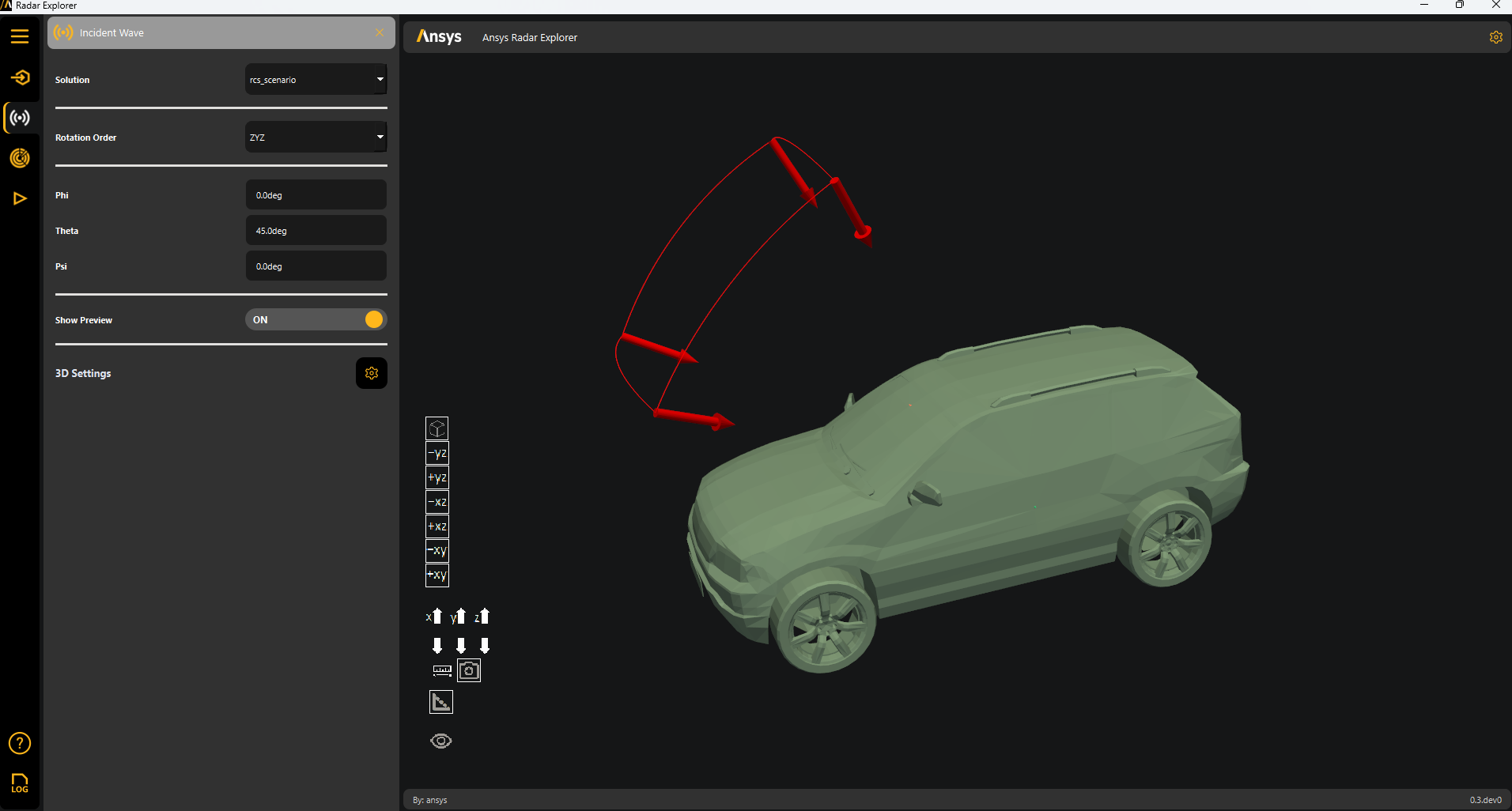
Incident wave panel#
Go to the Incident Wave panel from the left sidebar.
Use this panel to rotate the model so it aligns with the radar’s main direction of incidence and to visualize the radar’s incidence and observation domains around the chosen center.
This tool uses Euler (ZYZ) angles. Control orientation with these three parameters:
Phi (ϕ): Rotate about the global Z axis.
Theta (θ): Rotate about the intermediate Y′ axis (after ϕ).
Psi (ψ): Rotate about the final Z″ axis (after ϕ and θ).
All rotations follow the right-hand rule.
Set Show Preview to ON to display incident wave arrows in the plotter window:
Note
The arrows change based on the mode selected in the Mode Select panel.
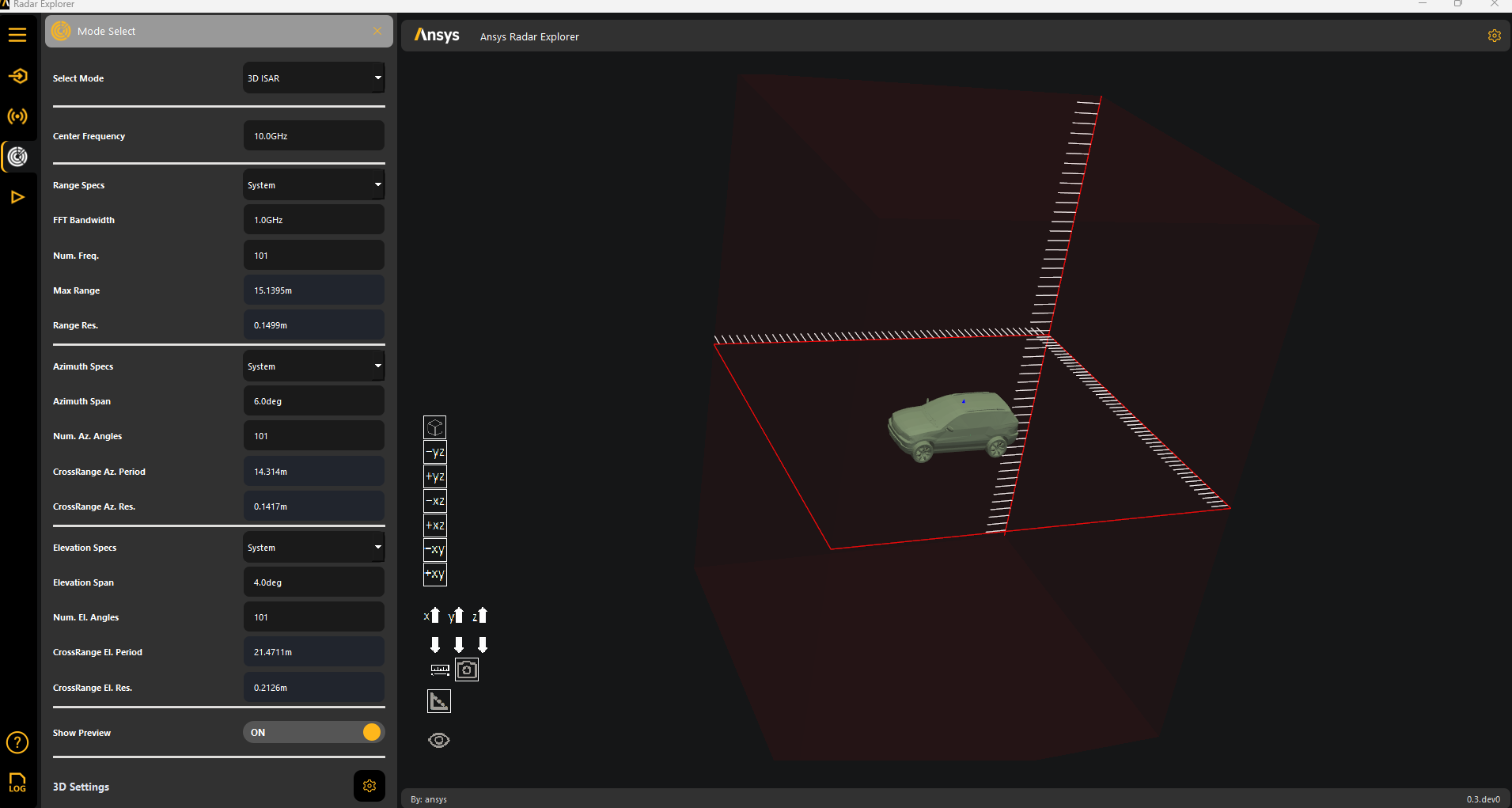
Mode select panel#
Go to the Mode Select panel from the left sidebar.
For Select Mode, choose one of the following solve modes:
Range Profile
2D ISAR
3D ISAR
Set Show Preview to ON to display incident wave arrows in the plotter window:
Solver setup panel#
Go to the Solver Setup panel from the left sidebar.
Configure the simulation parameters:
Ray Density: Number of rays to simulate for accuracy.
Number of Bounces: Maximum reflections a ray undergoes.
Cores: Number of cores to use. Using more cores speeds up simulations but might reduce accuracy.
Fast Freq. Looping: Whether to enable faster simulations at the cost of reduced accuracy.
PTD correction and UTD Ray: Whether to enable PTD and UTD in the SBR+ simulation.
Interactive: Whether to enable solving in graphical mode. When set to OFF, the simulation runs in non-graphical mode, thereby avoiding user interaction during simulation time, which might invalidate the simulation.
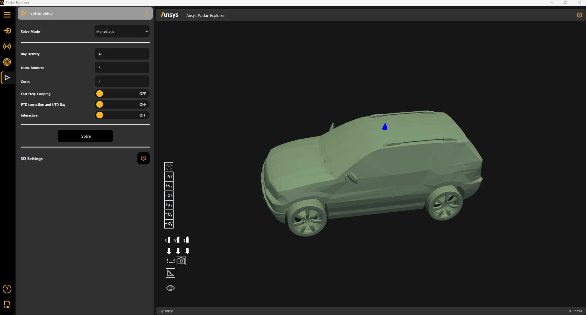
Click Solve to run the analysis.
After the simulation finishes, the system automatically extracts and loads the computed RCS data.
Check the output logs for any warnings or errors generated during the simulation.
After solving, the menu makes two additional panels available for 3D and 2D postprocessing. For more information, see 3D Postprocessing and 2D Postprocessing.